A Beginner’s Guide to Data Science in Python

Introduction

Python is quick to learn for beginners, but can still get things done for experienced data scientists because of its flexibility. If you have a data science problem that you need to tackle, Python can probably do it with one of its many external libraries. It’s important to know that Python is not always the best language for dealing with certain problems—it has far less functionality for traditional statistical modeling than R, STATA, or SAS, for instance—but it makes the learning curve easier to climb as a data scientist when you only have one language to deal with.

FIND SCHOOLS

Python Basics

There are a ton of lovely little beginner’s guides to Python out there. I like this, and this one, for instance, and Python also has a solid introduction to the language on its wiki. This guide focuses more on the data science side of things, where many of the tools come from outside libraries (called packages or modules in Python, depending on where you are in the hierarchy). We’ll get to that in a moment. But first we need at least a quick run-down of Python and its basic quirks, terminology, and functionality. Python has just about everything you would expect in a flexible programming language. It takes all the normal kinds of information, from intergers and floats, to strings and Boolean truth values. Python also has series of more complex data structures for when you need to do something more involved. Let’s take a look:

In [7]: an_integer = 3 a_float = 3.0 #Floats are used to store decimals a_string = ‘3’ a_bool = 3==3 print(‘An integer:’, an_integer, ‘… a float:’, a_float, ‘… a string:’, a_string, ‘… and a Boolean value:’, a_bool) # You can do math with integers and floats print(‘An integer plus a float? Yep!’, an_integer + a_float) # But not with a string print(‘Whoops’, an_integer + a_string) An integer: 3 … a float: 3.0 … a string: 3 … and a Boolean value: True An integer plus a float? Yep! 6.0 ————————————————————————— TypeError Traceback (most recent call last) <ipython-input-7-de1230c8fd30> in <module>() 11 12 # But not with a string —> 13 print(‘Whoops’, an_integer + a_string) TypeError: unsupported operand type(s) for +: ‘int’ and ‘str’ In [8]: # But you can add two strings together print(‘Concatenation!’, a_string + a_string) Concatenation! 33 In [18]: # You can store things in a list, even if they aren’t the same kind of thing a_list = [an_integer, a_string, a_string, a_float, a_bool] # Sets store unique items, so it will only keep one instance of each duplicate in our list a_set = set(a_list) # Dictionaries link a key to a value a_dict = {‘An integer’: an_integer, ‘A float’: a_float, ‘A string’: a_string, ‘A Boolean print(‘ The list:’, a_list, ‘\n The set:’, a_set, ‘\n The dictionary:’, a_dict) # The \n adds a new line to make this pretty The list: [3, ‘3’, ‘3’, 3.0, True] The set: {True, 3, ‘3’} The dictionary: {‘An integer’: 3, ‘A float’: 3.0, ‘A string’: ‘3’, ‘A Boolean value’: True}

You can pull information back out of these data structures by specifying what you want with square brackets. If you are interested in the first element of our list, we can simply write a_list[0], which tells Python to return the first value in the list (Python counts from 0). This is called slicing, and it works for a whole range of data types, including strings. If you wanted to do the same with a dictionary you would call the “key” of the first element, at which point Python would return the value.

In [20]: print(a_list[0], a_string[0], a_dict[‘An integer’]) 3 3 3

Python also comes with the regular set of conditional and looping functionality. Just be aware that the language has some pretty quirky syntax. Gone are the curly braces. Instead Python tracks nested syntax with whitespace. You must indent the content of your conditionals and loops, or it will return you an error.

In [27]: # You have your choice of if-statements, else-statements, and else-if statements if an_integer > 2: print(an_integer, ‘is bigger than 1!’) elif an_integer <= 1: print(an_integer, ‘is smaller or equal to 1′) if a_string == ’33’: print(‘It matches!’) else: print(‘No match on the strings’) # You also have for-loops and while-loops for i in range(0,3): print(i) i = 0 while i < 3: print(i) i += 1 # Python doesn’t use the usual i++ notation 3 is bigger than 1! No match on the strings 0 1 2 0 1 2

A Beginner’s Toolkit

The really simple way to think about data science is to say that it deals with two kinds of problems: (1) finding patterns in data where there is no clear outcome variable and (2) finding patterns in data (and making predictions about them) where there is a clear outcome variable.

We tackle the first kind of problem with unsupervised learning and can usually think of it as a problem of how to cluster the data we do have. The second kind of problem is either an issue of classification or regression, depending on the kind of variable. We use supervised learning techniques to solve this kind of problem. Friendly note: the “supervision” part of a machine learning algorithm specifically refers to whether or not we have data on an outcome variable. When we have an outcome variable we’re interested in, we call it supervised learning. When we don’t have that data, we call it unsupervised learning. Python’s scikit-learn module has an extensive collection of machine learning algorithms, so we’re going to use that here.

Clustering

There are a bunch of unsupervised learning techniques out there, but many of them boil down to different ways of finding clusters in data. We’re going to focus on that here. If you came here looking for a run down of dimensionality reduction, you’re out of luck!

K-Means Clustering

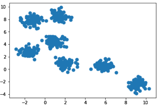
Let’s talk about k-means clustering, one of the most common clustering algorithms. The k-means algorithm works to find k clusters, so that each member of a cluster is closer to the mean point within the cluster they were assigned to than they are to the mean point of any other cluster. This makes it super helpful when you’re exploring a dataset. I’ll make some blobs of data to make the concept a little more obvious.

In [21]: %matplotlib inline import matplotlib.pyplot as plt from sklearn.datasets.samples_generator import make_blobs # We’ll make “blobs” using the make_blobs() function in sklearn X, y = make_blobs(n_samples=500, centers=7, random_state=0, cluster_std=0.50) plt.scatter(X[:, 0], X[:, 1], s=50);

So we have seven pretty obvious clusters here. It may not always be obvious how many clusters there are in your data, so let’s go ahead and run k-means clustering, telling it to find 3 clusters. Afterwards, we’ll run it again and tell it to find all 7 clusters.

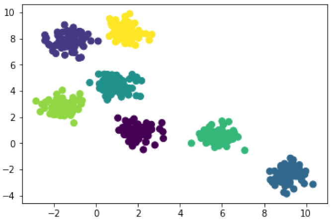
In [4]: from sklearn.cluster import KMeans model_3 = KMeans(3) # 3 clusters model_3.fit(X) cluster_3 = model_3.predict(X) plt.scatter(X[:, 0], X[:, 1], c=cluster_3, s=50); In [5]: model_7 = KMeans(7) # 7 clusters model_7.fit(X) cluster_7 = model_7.predict(X) plt.scatter(X[:, 0], X[:, 1], c=cluster_7, s=50);

You’ll notice that k-means does a pretty good job in each case. Obviously it’s a better fit when it looks for 7 clusters, but the model with just 3 clusters produces reasonable groupings too. It takes some familiarity with your data and some domain knowledge to make a meaningful choice for k (i.e. the number of clusters).

Hierarchical Clustering

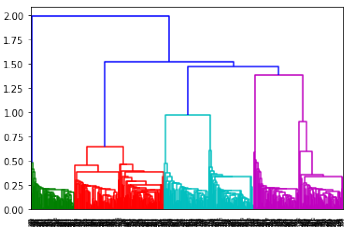
Another way you might want to look at this data is through hierarchical clustering which works from the bottom-up to build a tree where data points are clustered at different levels. This sounds a little abstract, but the process isn’t all that complicated. Starting from a situation where every data point is in its own cluster, hierarchical clustering then takes the closest two clusters (there are different ways of measuring distance) and combines them into a single cluster. This process repeats itself over and over again until every data point belongs to the same cluster. Using the same blob data we created a moment ago, the resulting tree looks like this:

In [8]: from scipy.cluster.hierarchy import dendrogram, linkage hmodel = linkage(X) dendrogram(hmodel);

Reading a dendogram isn’t all that informative, but it does illustrate the process. The individual data points are at the bottom, and each step in the linking process is represented by a connection at a higher point. The algorithm stops with the link at the top. I used scipy’s implementation of hierarchical clustering there, but I’m going to switch right back to scikit-learn. The reason is both simple and a little silly:

scikit-learn makes it very easy to know which of k clusters a data point belongs to. You just specify how many clusters you want when you fit the model. scipy can do this too, but it’s slightly more involved and a bit less intuitive: we need to “cut” the tree at a specific point to return the cluster labels.
In a cruel twist of fate, though, scikit-learn makes it hard to plot the resulting dendogram. In scipy, this is simple.

I can’t tell you why we can’t have the best of both worlds, but there you have it. Now let’s ask scikit-learn to run hierarchical clustering and sort our data points. Again, I’ll ask it to sort them into 3 clusters and then 7 clusters, so we can compare the results with our k-means clustering algorithm above. (As an aside, just know that scipy has a great collection of tools itself, so you’re not doing it wrong if you prefer it to scikit-learn.)

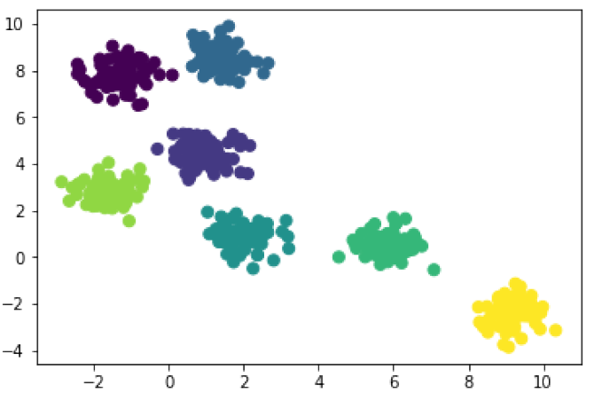
In [6]: from sklearn.cluster import AgglomerativeClustering hmodel_3 = AgglomerativeClustering(n_clusters=3) # 3 clusters hcluster_3 = hmodel_3.fit_predict(X) plt.scatter(X[:, 0], X[:, 1], c=hcluster_3, s=50); In [9]: hmodel_7 = AgglomerativeClustering(n_clusters=7) # 3 clusters hcluster_7 = hmodel_7.fit_predict(X) plt.scatter(X[:, 0], X[:, 1], c=hcluster_7, s=50);

The results are identical when we ask our algorithms to look for 7 clusters. That’s what you want to see when the blobs are clear like this. And you’ll notice that when they are looking for just 3 clusters hierarchical clustering and k-means clustering disagree a little. That’s fine, and we would probably have to check with our domain knowledge to decide which algorithm is working best. And the results can vary even more! Hierarchical clustering works differently depending on the way distance is calculated, and how links are chosen. I used the default settings for these models, Euclidean distance and Ward linkage, because they tend to work for a wide variety of data. But you can mix-and-match your settings depending on the quirks of your data. Just be sure to do some technical reading so that you make intelligent choices.

Classification and Regression

Now say you’re interested in predicting what category a data point might represents. Maybe you’re interested in sorting winning stocks from losing ones, or all-star athletes from average ones. These are classification problems. Classification also comes with a partner concept: when the task isn’t to sort data points into categories, but to sort them according to a continuous variable, we use regression techniques. So if instead you wanted to know the likely value of a house, the population growth in a country, or the number of reviews a product can be expected to get on your website, you have a regression problem. Most classification techniques have versions that handle regression too, so it isn’t much of a hassle to keep these straight. Once you know what kind of outcome variable you have, you can just apply the right version (in a smart way, hopefully) and you’re off to the races! There are a bunch of different classification and regression techniques, so we can’t touch on them all. We’ll get you started with the k-nearest neighbor algorithm and random forests (bunches of decision trees averaged together). Again, we’ll use the implementations in scikit-learn, which are pretty good.

K-Nearest Neighbors

The k-nearest neighbors algorithm is very simple. The idea is to make classification and regression decisions for new data based on the values held by the most similar data points in our dataset. The algorithm begins by finding the k data points that are closest to the data point you want to classify. These are the neighbors in k-nearest neighbors. For a classification problem the next step is to take a vote. The category that is shows up the most among the k neighbors “wins” and we use it to classify the new data point as well. In regression we take the average value of the k neighbors, weighted by how distant a data point is from our new case. Let’s see it in action. We’ll practice with a classic dataset on breast cancer from the University of Wisconsin. The outcome variable is pretty simple: tumors are either malignant or benign. So we’re going to be doing classification rather than regression. I am going to use the pandas module to put the data into a dataframe, which will just make it a little easier to navigate and explore. Pandas also has Python’s go-to set of statistical tools. We’ll talk about that a little more below.

In [13]: from sklearn.datasets import load_breast_cancer from sklearn.neighbors import KNeighborsClassifier import pandas as pd data = load_breast_cancer() cancer = pd.DataFrame(data.data, columns = data.feature_names) # Makes a dataframe from cancer[‘diagnosis’] = data.target cancer.head() # Shows us the first few rows of data

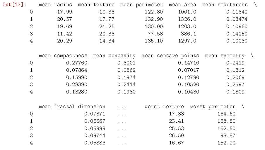
As you can see, the dataset has 30 predictors which relate different aspects of a tumor. We know whether each tumor was diagnosed as malignant or benign, so we move forward by splitting the data into a training set and a test set. The training set is used, like you might have guessed from the name, to train the k-nearest neighbors model to predict cancer diagnoses. Once the training is over and done with, we use the test set to see how well the model can predict the diagnosis in new cases. scikit-learn has a convenient function to split datasets in this way. It uses 75% of the cases for training, and saves the other 25% for testing.

In [16]: from sklearn.model_selection import train_test_split # This function splits our data into predictors and outcomes for both training and test X_train, X_test, y_train, y_test = train_test_split(cancer.drop(‘diagnosis’, axis=1), cancer.diagnosis, knearest = KNeighborsClassifier(n_neighbors = 5) # 5 nearest neighbors, in this case knearest.fit(X_train, y_train);

The model has been fit. Let’s see how well it actually does predicting new cases:

In [15]: knearest.score(X_test, y_test) Out[15]: 0.93706293706293708

The model is right in its predictions 93-94% of the time! Other approaches may do even better. In the next section we will see if a basic random forest can out-perform our basic k-nearest neighbors model here.

Random Forests

Random forests have gotten a lot of attention over the past few years because they have become absurdly good at dealing with a wide range of problems, considering the very simple idea at their core. A random forest is an ensemble method, which means that it takes something like an average across many individual models to make a prediction for a classification or regression problem. While any given model is likely to make some systematically flawed inferences because of quirky training data, it’s very unlikely that those mistakes are going to be repeated in other models with even slightly different training data. By blending a collection (an “ensemble”) of models together we get a composite view of the situation that performs better than any given model on its own. Random forests are an ensemble of decision trees, specifically, which work by partitioning data repeatedly according to an information criterion that indicates which division best separates cases by their value on the outcome variable. You can think of decision trees like the machine learning version of “Guess Who” or “Twenty Questions”.

If we care about who develops cancer, we can first divide smokers from non-smokers, and then within those groups divide people who exercise from those who don’t, and then within those groups divide people who have a healthy diet from those who don’t, and so on. The result is a tree that you can follow to make an informed prediction about where a particular case will fall. With a random forest we estimate a whole bunch of decision trees, each slightly different from the last, whether because we change the parameters it can decide over, or by using bootstrapping to change the sample for each tree. An averaging process helps to make final predictions for the forest as a whole. scikit-learn has a solid implementation of random forests here, too. (You might be sensing a trend, but just know that scikit-learn is not the only useful package for data science in Python…it’s just convenient having so much in one place.) Let’s give it a try with the breast cancer data.

In [19]: from sklearn.ensemble import RandomForestClassifier forest = RandomForestClassifier(n_estimators=50, random_state=0) # The more estimators forest.fit(X_train, y_train); forest.score(X_test, y_test) Out[19]: 0.965034965034965

You can see that the random forest is a little more accurate than our k-nearest neighbors model from above. It gets the right diagnosis for another 3% of the cases. We can actually test these on the blobs we used for clustering, since the make_blobs() function creates an outcome variable.

In [24]: # Train-test split the blob data X_train_blob, X_test_blob, y_train_blob, y_test_blob = train_test_split(X, y, random_state=0) # Estimate our k-nearest neighbors model knearest_blob = KNeighborsClassifier(n_neighbors = 5) knearest_blob.fit(X_train_blob, y_train_blob); # And the random forest forest_blob = RandomForestClassifier(n_estimators=50, random_state=0) forest_blob.fit(X_train_blob, y_train_blob); # And let’s look at the results! print(“K-Nearest Neighbor:”, knearest_blob.score(X_test_blob, y_test_blob)) print(“Random Forest:”, forest_blob.score(X_test_blob, y_test_blob)) K-Nearest Neighbor: 1.0 Random Forest: 0.992

And! … statistics – It’s important to realize that you can’t just throw old-school stats out the window when you’re a data scientist. Classification and regression models don’t just vary by how well they can make predictions. They also vary by how easily we can interpret them. So for instance, consider a really simple example:

Deep neural networks have become an extremely powerful tool set in a very short time, but it’s still incredibly hard to explain to someone why it interprets given data in the way it does. The same can be said of random forests, to a certain extent. This may not seem like much of a problem if you only care about maximizing ad revenue or making the best possible recommendations to users. But if your models are going to inform business strategy or government policy it becomes important to be able to communicate how the models are doing their work. Try not to see every problem as a newfangled machine learning problem. Sometimes, good ol’ statistics is the best way to solve a classification or regression problem, even if you have to sacrifice some predictive power. Most of your statistical needs are going to be filled by the pandas and statsmodels modules. Just be aware that for hardcore statistical models you may need to use R, STATA, or SAS. With the Wisconsin cancer data we could run a simple logistic regression, for instance. A simple logistic regression classifier is already implemented in scikit-learn, one that we can deploy using code that is very similar to what we have already seen. The module isn’t ideal for a full statistical analysis, but it will do for a classification job in a pinch.

In [26]: from sklearn.linear_model import LogisticRegression logit = LogisticRegression() logit.fit(X_train, y_train);

You can see below that if you want to pull out the fitted intercept and coefficients for the model, it’s not very user-friendly. Remember: the scikit-learn implementation isn’t designed with regression tables in mind.

But finding out how well the model does at prediction is very inuitive. And it does pretty well! Better, in fact, than the k-nearest model did, and nearly as well as the random forest.

In [30]: logit.score(X_test, y_test) Out[30]: 0.95804195804195802

We’re Gonna Need a Bigger Toolkit

Think of this as the beginner-plus section. The issues below aren’t quite simple enough to fully explain in an introductory guide, but they are common enough that it’s helpful to mention here. So, if you run into a wall dealing with something like hierarchical data or relational data, just know that you’re not alone and you’re not hopeless. There are well-developed techniques for dealing with them. The short discussion here will give you some solid clues about where to start.

Hierarchical Data

Not all data look like what we’ve been dealing with so far. A really simple way to understand the problem is to think of the cancer data (and the blob data) as a table. You have variables stored in the columns, and an individual case in each row. So far we’ve assumed that each row is basically independent from the others. It doesn’t matter how big or how rough someone else’s tumor is, it isn’t going to change the size and roughness of another person’s tumor. Cancer just doesn’t work like that. This isn’t true for all data. The most common problem is that the data are hierarchical. By that I just mean that cases are bunched together in real life. One way to explain this is to think about student performance. You can obviously assume that each student is in their own little island and create a classification or regression model to predict their test scores. But this isn’t really true. Students sometimes share teachers, attend the same schools, live in the same school districts, and so on. The 30 students in Mr. X’s class share experiences that the 30 students in Ms. Y’s class do not, and vice versa. And the 10000 students who live in a good school district might get better overall education than 10000 students who live in a worse school district.

There are a number of well-known ways of dealing with this using fixed- or random-effects and multi-level models. (You don’t need to know what any of that means unless you find yourself needing to deal with this kind of data.) The more complex machine learning models, like random forests or deep neural networks can also handle this kind of data without too much trouble. Computer vision applications, for instance, face this kind of problem all the time. You need the computer to not just recognize a single pixel, but the shape nearby pixels come together to form if it’s going to classify images or keep a car in its lane.

Relational Data (Networks)

The other kind of non-independent data that you will probably run into in short order is what we call relational data. These are things where the data points are connected to each other in a network. If you want to deal with data from Twitter, Instagram, Facebook, Snapchat, LinkedIn, and so on then you are going to care about the structure of the relationships on there. Facebook Research actually drives that point home really well. If you’re interested in how many people are going to “like” or “share” a story on the platform it isn’t enough to just analyze the story itself (e.g. its title, its blurb, its source, its content, etc.). You need to know who shares the story at time zero, and who can see it after it gets shared. If they only share it with one person, it can only spread to one person at time one. If they share it to ten thousand people, that number can be dramatically bigger.

Research at the tech giants and at universities keeps showing that information travel (and cascades!) down friendship networks. Python has a solid set of modules to deal with relational data, igraph and NetworkX being the two most prominent.

Textual Data

A lot of the data out there today is basically just text. We have tweets, comments, articles, and so on. There are some fancy things we can do with that pile of information, and Python does them well. Natural language processing (NLP) is the field of research specifically concerned with how to help make sense of text data. This is another HUGE area in data science, but I’ll give you the sneak preview.

The main piece of data in NLP is called a token, which is usually a word. “Cat”, “AI”, and “lavender” are all tokens. But technically, so is anything else you can type without hitting the space bar, like “jifoewa” or “zzzz”. There are a bunch of different ways to make tokens useful. The simplest way is to use what we call n-grams and track how often they are used over time. An n-gram is a set of N tokens that appear side by side in a text. So a 1-gram is one token, a 2-gram is two tokens that appear together, a 3-gram is three tokens that appear together, and so on. The Google n-gram viewer is a fun place to figure out how these work, and how they can matter. You can track how often terms are used to see spikes in interest over time. We can combine this with sentiment analysis or topic modeling to understand what a text is talking about and what kind of valence is there.

Someone tweeting about “united nations” and “first nations” are clearly dealing with politics. Topic modeling will notice that. With sentiment analysis we can figure out if they see the issue in a positive or negative light (among other things). Practically speaking, you can use this to understanding not just what is trending on social media, but how people feel about it. You will also see this used to connect the textual content of a product review and its sentiment to the star rating given in the review—so a business can understand what about its offering is leading people to review it the way they do. Analysts also work the other way around, using a product’s characteristics to predict the sentiment of its reviews (a lot of data science competitions work like this, too). For NLP in Python we use the nltk and gensim modules mainly.

And that’s it for this guide!

FIND SCHOOLS

Additional Programs

Other Degrees and Certificate Programs

Career Guides – How to Become:

Salary Guides

Articles

FAQ

Social Good

Data Science in Industry

Data Science Training Toolkits

More Resources & Helpfull Guides

Top Picks